Geometry of Reflection: How Models Move Through Meaning

When frontier LLMs “think again,” their answers don’t just change, they move.

Dec 06, 2025

What follows is our attempt to treat that movement not as metaphor, but as geometry.

In Part I – Geometry of Reflection: How AI Models Think in Curved Space, we treated reflection as motion on a hypersphere. We watched models rethink their own answers and traced those moves as curved paths on a normalized semantic space—an operational manifold defined by a fixed external encoder. By measuring curvature, angular velocity, and path efficiency, we found that different architectures don’t just give different answers; they trace different shapes of thought.

In Fingerprint of Thought: When Models Iterate, What Do They Reveal?, a kind of Part 1.5, we shifted to the surface: how similarity, length, and coefficient of variation behave across eight loops of reflection and regeneration. That piece was about morphology and stability—collapse vs explosion, capability vs convergence—read directly from the text.

This essay steps back into the geometry.

Here we:

Scale the experiment up to 11 models × 8 scaffolds × 13k prompts totaling 104,896 embeddings
Embed all outputs into a single operational manifold using a third-party encoder, and
Treat reflection explicitly as a discrete dynamical system.

Formally, the reflection operator Φ takes the previous embedding x_i, the model M, the reflection style s, and the prompt context θ, and returns the next point in the trajectory:

From there we can measure reflection as motion: trajectories that show large early reframes, then shrinking steps and stabilization across loops, with consistent signatures across models and scaffolds.

If you remember one thing, let it be this:

Reflection is a discrete dynamical system on a shared operational manifold defined by a single external encoder.

When we talk with LLMs, we’re not just giving them prompts, we’re stepping into a shared space of meaning, where our words and theirs reshape each other with every additional prompt in the conversation.

The Expanded Experiment

For this second expanded experiment, we scaled up and cleaned up.

11 models from 6 provider families

Anthropic – Claude 4.5 family
OpenAI – GPT-5, GPT-5.1
Google – Gemini 2.5 Flash Lite, Gemini 3 Pro
xAI – Grok-4, Grok-4.1-Fast
DeepSeek – V3.1 Terminus
Moonshot – Kimi K2-Thinking

13K prompts, across:

philosophical and meta-philosophical questions
ethical dilemmas
technical and scientific problems
financial, medical, and health questions
creative writing and songwriting
meta-cognitive questions about thinking itself

8 reflection styles

notice_emotion
notice_language
notice_uncertainty
notice_contradiction
notice_bias
notice_honesty
challenge_accuracy
none (no reflective instruction at all)

8 loops per run

Initial answer (loop 0)
Up to 7 reflective steps (loops 1–7)

Total: 104,896 reflection loops.

For each trajectory {x_0, …, x_7} we compute:

Per-step cosine shift
Δcos(i) = 1 − cos(x_i, x_{i−1})
Per-step distance (“effort”)
Δ(i) = ||x_i − x_{i−1}||
Net displacement
D = ||x_7 − x_0||
Path length
L = Σ_{i=1..7} ||x_i − x_{i−1}||
Global tortuosity (curvature-like)
τ = L / (D + ε) (with ε to avoid division by zero)
Local discrete curvature (for interior points x_i, 1 ≤ i ≤ 6)
- First difference: Δx_i = x_{i+1} − x_i
- Second difference: Δ²x_i = x_{i+1} − 2x_i + x_{i−1}
- Curvature estimate: κ_i = ||Δ²x_i|| / ||Δx_i||²
High κ_i means a sharp turn; low κ_i means smooth motion.
Semantic variance of the trajectory: the spread of {x_0, …, x_7} around their centroid.
Stabilization loop
The first loop k where per-step cosine shift satisfies:
Δcos(k) < 0.05 and remains below small threshold for all subsequent steps.
Intuitively: the first time the trajectory’s moves become small and stay small.

Each reflective run becomes a geometric object with:

a scale (how far it travels),
a shape (how straight or loopy),
a rhythm (how quickly it shrinks), and
a stopping time (when it stabilizes).

Two Geometric Spaces

Before we go any further, we need one critical distinction. The rest of this essay depends on keeping these two spaces separate: one is where we measure dynamics, the other is where we see structure.

We are actually working with two geometric objects.

(1) The high-dimensional embedding space

All trajectory points x_0, …, x_7 live here.
This is the space of the external sentence encoder (for example, a 4,096-dimensional real vector space, which we’ll just call R^d).
In the white paper we instantiate this with E5-mistral-7b-instruct as a universal encoder, but any fixed sentence embedder would define a similar operational manifold.
This is where the reflection operator Φ acts:
x_{i+1} = Φ(x_i; M, s, θ)

(2) The 2D UMAP projection

A compressed view of that high-D space in R^2.
Used only for visualization and coarse topology.
UMAP preserves local neighborhoods reasonably well but distorts global distances.

When we say “the manifold”, we mean the high-dimensional embedding space unless explicitly noted.
When we talk about “the map” or “UMAP layout,” we’re talking about the 2D projection.

That distinction matters: the dynamics and curvature live in the high-D space; the pretty pictures and some of the style/provider topology live in 2D.

We take all embeddings {x_0, …, x_7} for all models and runs and feed them through UMAP, yielding a 2D projection. That 2D map is our semantic atlas of the operational manifold.

Our style/provider variance decompositions for “the map” are done in this 2D projection. So those percentages describe the projection layout, not the underlying high-D geometry.

Now we zoom out and make the things visible.

One Continuous Cloud

This plot is excellent for seeing shared geography and coarse separation, but it’s not where we’ll make our strongest causal claims.

Read this as geography, not measurement. Proximity here means “similar under the external encoder,” not “true distance inside any particular model.” The map is a diagram of outputs in a shared coordinate frame, not a window into internal representations.

With that in mind, the operational manifold has a dense core, with filamentary arms and peripheral lobes. It looks less like a random cloud and more like terrain: continents of high density, plus corridors that lead outward.

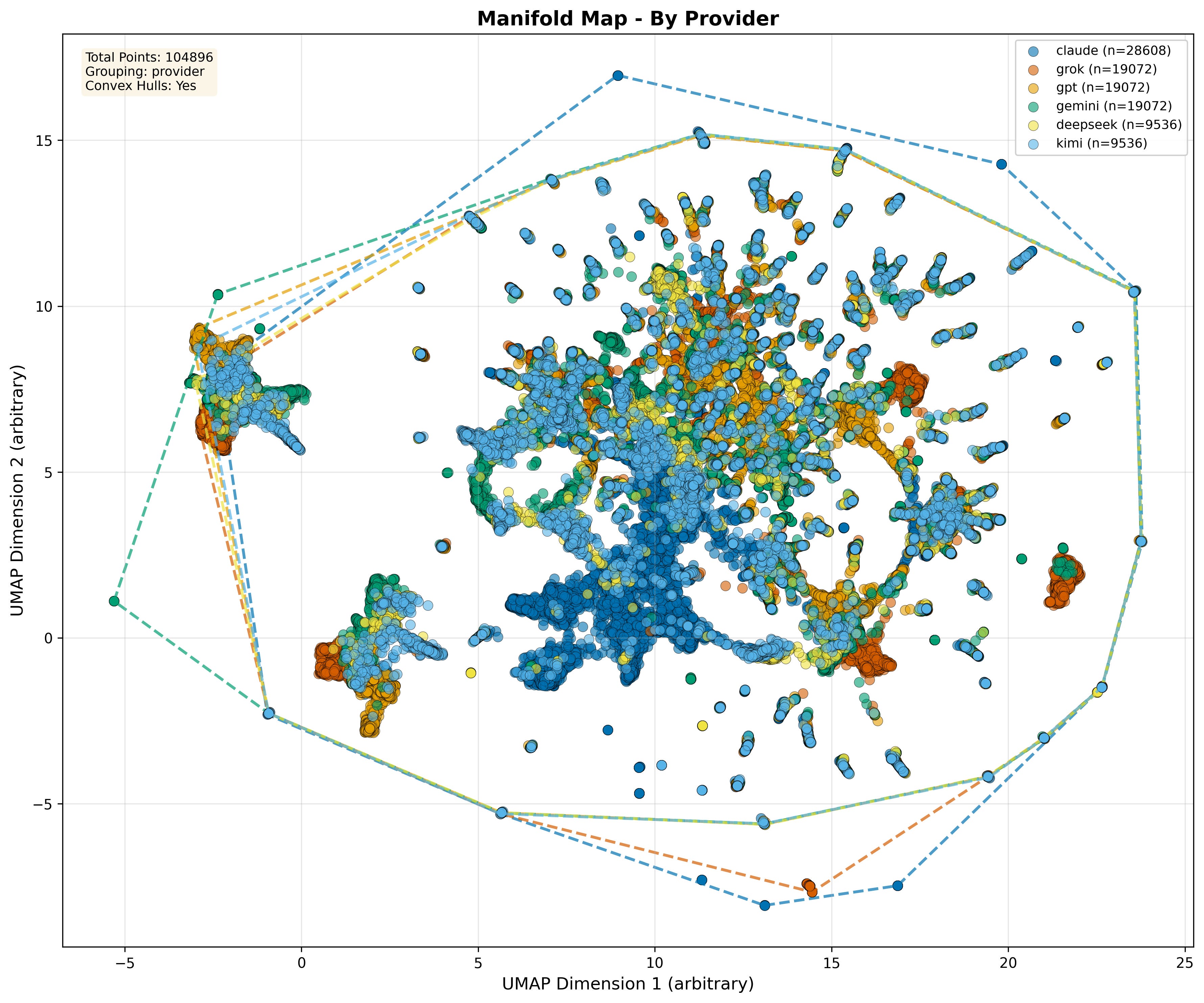
Manifold Map by LLM Provider. 2D UMAP projection of 104,896 reflected outputs embedded by a single external encoder, recolored by LLM provider. Providers overlap on the same semantic terrain. Differences appear mainly as density and reach (convex hulls), not clean provider-exclusive regions.

The map is colored by provider. Two things are worth noticing without over-interpreting the projection. First, most providers share the same central terrain. They are not living on different planets. Second, providers still leave distinct fingerprints in where they spend density and how far their hulls reach.

Providers overlap heavily on the same terrain, differing more in where they concentrate and how far they reach into satellites and low-density bridges.

If you draw convex hulls, the overlap becomes hard to ignore. Providers differ in preferred zones and spread, but the hulls intersect heavily. So when someone asks, “Does provider X think in a totally different world than provider Y?” the answer, at least in this operational manifold is: no. The differences are real, but they show up as where mass accumulates and how far it extends, not as disjoint semantic universes.

This is important but subtle:

It does not mean internal representations are identical across providers.
It means that when their outputs are projected through the same encoder, they occupy overlapping regions of a common semantic frame.

Now for the subtle part. When people look at plots like this, they often interpret blank space as “semantic emptiness.” But whitespace in a UMAP map is best read as absence of sampled outputs, not absence of meaning. Our prompt set and reflection scaffolds concentrate trajectories into a handful of high-density neighborhoods. Regions that look empty are often just low-density zones under this particular experimental distribution.

UMAP also plays a role. It preserves local neighborhoods reasonably well, but it can distort global distances. So when you see a “satellite” blob, you should treat it as a region the experiment visits less frequently and that the projection has pulled apart, not automatically as a disconnected semantic island. With broader prompt coverage, you’d reasonably expect some of the gaps and apparent separation to soften further.

The point of this figure is not to prove a topological theorem about connectedness. It’s to establish the stage: the outputs we’re measuring—across all models, prompts, and reflection loops—live in a single shared coordinate frame.

Coloring by Reflection Style

Now color by reflection style and things pop.

Styles like notice_emotion and notice_uncertainty push outputs toward more peripheral, exploratory regions.
Styles like challenge_accuracy and notice_bias concentrate nearer dense, central bands.
The none condition stays tucked close to the core.

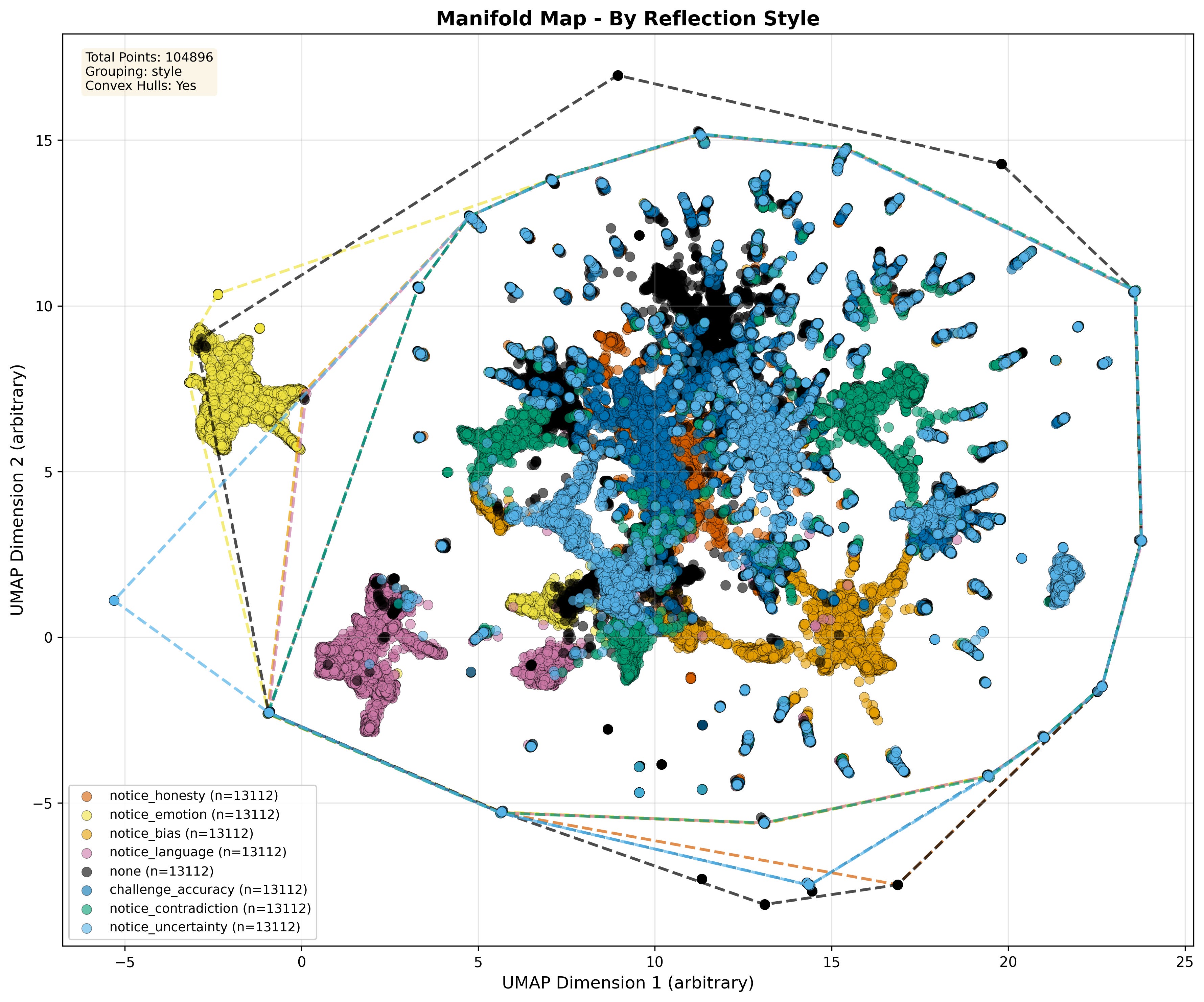
Manifold Map by Reflection Style. 2D UMAP projection of 104,896 reflected outputs, recolored by reflection style. Convex hulls outline each style’s territory; the visualization illustrates the style-dependent organization of the operational manifold used in this study.

If you do a variance decomposition on pairwise distances in this 2D projection, you find that: Reflection style explains more of this projected layout than provider does. In this 2D view, style accounts for roughly twice as much of the layout as provider identity (≈69% vs ≈34% in our full analysis), so styles line up more cleanly into regions than providers do.

This does not mean “style is more important than architecture in absolute terms.”

The right way to read it:

Gaits (step sizes, curvature, stabilization) are mostly architectural.
Fields (which regions are populated, under this projection) are strongly influenced by reflection style.

Architecture sets how the model walks.
Style determines which parts of the map that walk tends to pass through.

In the next essay, we’ll switch from “where points sit” to “what forces steer motion,” and show why reflection style behaves less like a label and more like a field over that shared terrain.

Reflection as a Discrete Dynamical System

For each run, the process looks like this:

You ask a question.
A model M answers (loop 0).
You show it that answer plus a reflection style s (“notice emotion”, “challenge accuracy”, or none) and ask it to respond again (loop 1).
You repeat up to loop 7.

Each response is converted into a point x_i ∈ R^d by a single external embedding model applied uniformly across all providers.

So every reflective run becomes a trajectory:

x_0 → x_1 → x_2 → … → x_7

We can write the dynamics as:

x_{i+1} = Φ(x_i; M, s, θ)

where:

M = model family / provider
s = reflection style / scaffold
θ = prompt and task context
Φ = the reflection operator: “given what I just said, how do I revise it?”

We never see Φ directly. We only see its footprints: the positions x_i and the transitions x_i → x_{i+1}.

And we are explicit about the space this lives in:

We treat the embedding space as an operational manifold: a semantic measurement space defined entirely by the external encoder, not by any model’s internal activations.

We are not claiming all models literally share an internal geometry; we are claiming that, when their outputs are projected through the same encoder, their reflective behavior becomes comparable in a shared coordinate frame.

Universal Two-Phase Pattern

Across all 11 models and 8 styles, reflection follows the same temporal script.

Phase 1: The big reframe (0 → 1)

The transition x_0 → x_1 is always the biggest:

Per-step cosine shift peaks at loop 1.
Per-step distance Δ(1) is the largest of any step.
Local curvature κ_1 is often high: trajectories make sharp turns off the initial direction.

Semantically: the first reflective step is where the model goes,
“OK, given what I just said… here’s a different way to frame it.”

It doesn’t just polish; it repositions.

Phase 2: Annealing (1 → 7)

After that first jump, step size shrinks:

Δcos(i) and Δ(i) decay over loops, not perfectly exponentially, but monotonically on average.
By loops 5–7, most trajectories are making tiny adjustments.

Two-Phase Reflection Dynamics. Panel A shows the sharp 71% decline in per-step cosine shift after the initial reflection (semantic change). Panel B shows a 2.6× growth in semantic variance (response diversity) before stabilization. Shaded regions mark the exploration (blue) and drift (red) phases; black line = grand mean with 95 % CI.

At the same time:

Semantic variance of each trajectory grows by a factor of about 2.7× before plateauing.
Per-step shift drops by about 70% from early to late loops.
Net displacement keeps increasing, but with diminishing increments.
The stabilization loop falls, for most runs, between 3 and 6.

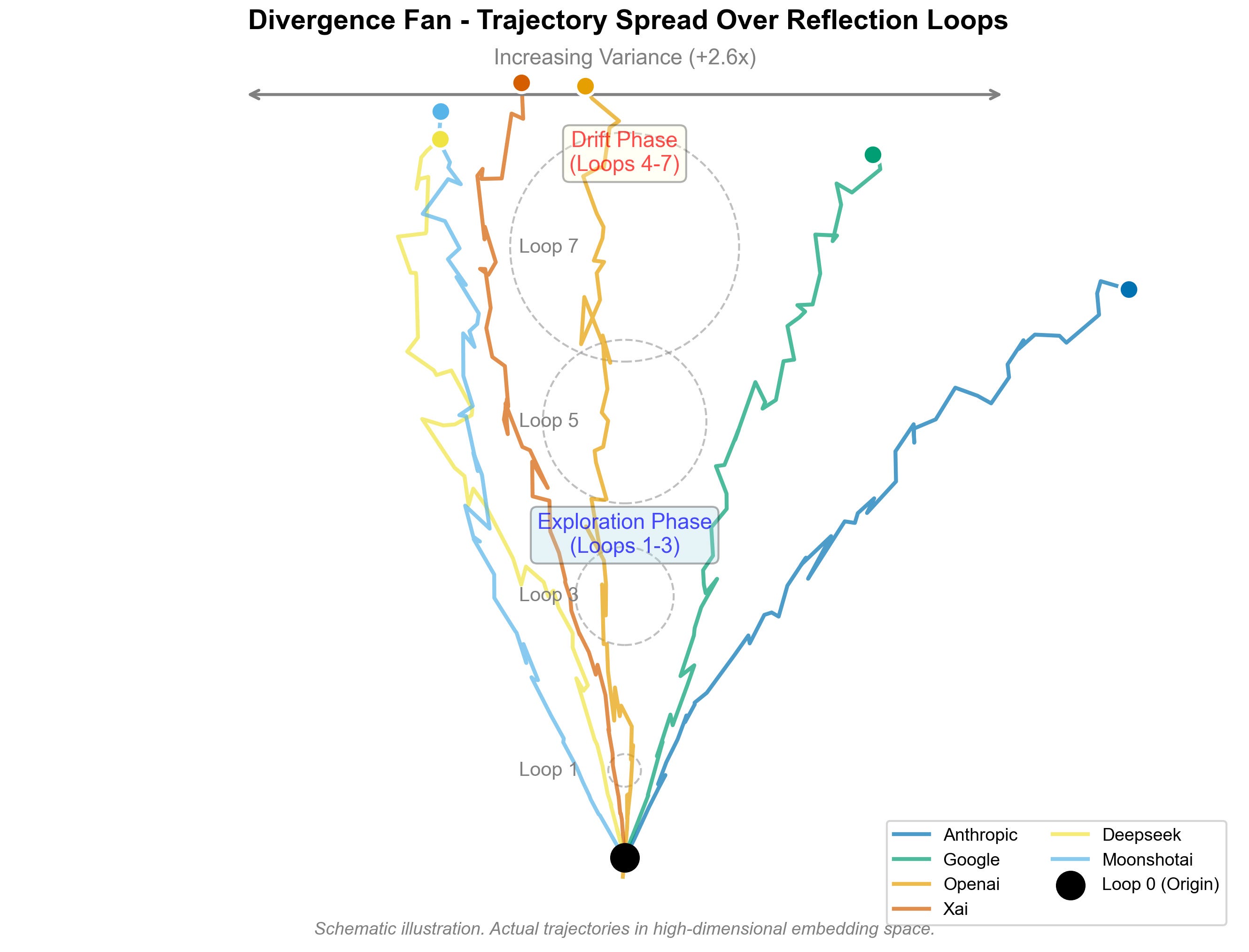
Divergence Fan of Reflection Trajectories. Each colored path shows the mean trajectory for a provider family, expanding during the exploration phase (loops 1–3) and diffusing in the drift phase (loops 4–7). Variance increases ≈ 2.6×, consistent with quantitative results in Figure 2.

So reflection trajectories show a characteristic exploration → drift structure:

Exploration: large, sometimes curved moves into new semantic territory.
Drift / annealing: smaller, smoother updates that settle into a local region.

Crucially:

Individual trajectories stabilize, they stop changing much.
But as a population, endpoints are more spread out than starting points: reflection increases global variance.

Reflection is not convergence on a single “true” point. It’s a diffusive flow where each run finds its own patch of stability.

Three Axes of Reflection Behavior

All those metrics are correlated, but not redundant.

When we look across all 13K runs and the ~105K embeddings, three main axes emerge:

(1) Local-change axis

Per-step cosine shift Δcos(i)
Per-step distance Δ(i)

These move together: trajectories with high cosine shift also have high distance. This axis captures how vigorously each reflection step moves.

(2) Exploration-radius axis

Semantic variance
Net displacement D
Path length L

These form a second cluster: longer paths and larger net displacement go with broader variance. This axis measures how far trajectories roam before settling.

(3) Curvature axis

Global tortuosity τ = L / (D + ε)
Local curvatures κ_i

This axis is more independent: you can have big radius but straight paths (ballistic), or modest radius but very loopy ones (ruminative).

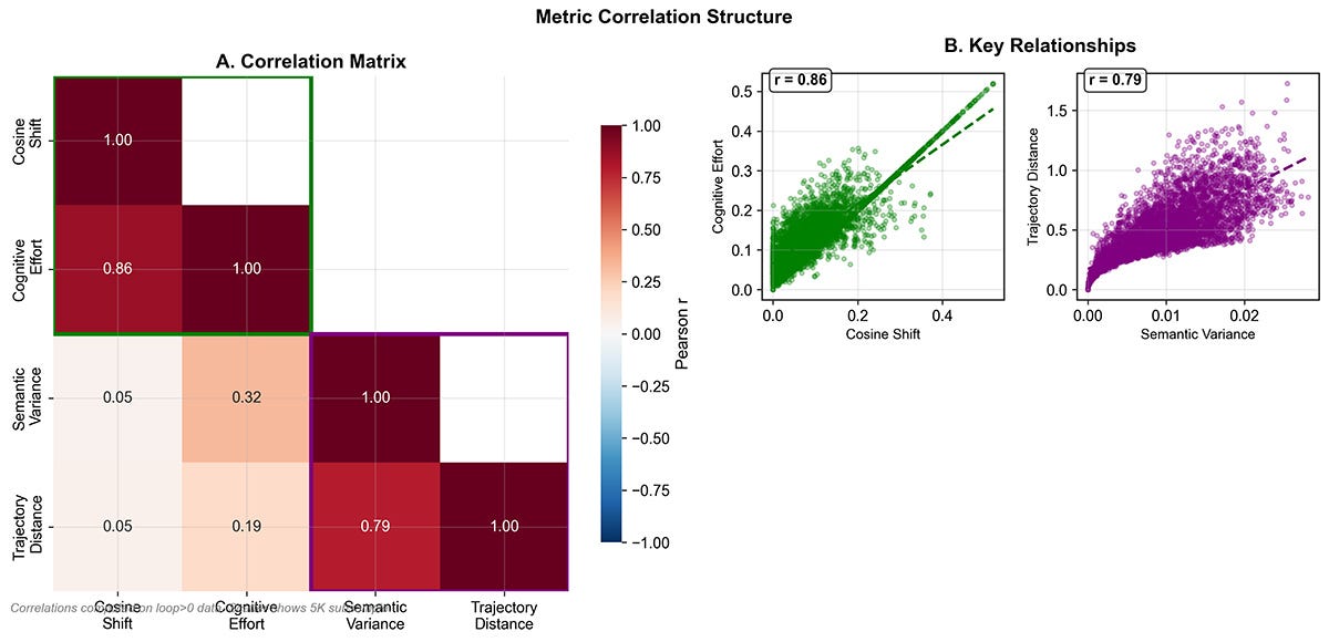
Metric Correlation Structure. Panel A shows strong coupling (r = 0.86) between cosine shift and cognitive effort, defining the local-change axis. Panel B shows trajectory distance correlating with semantic variance (r = 0.79), anchoring the exploration-radius axis. Together these relationships justify the three-axis decomposition introduced in this section.

So each reflective run can be roughly located in a 3D behavioral space. Three main axes emerge:

Local change: per-step cosine shift and distance (how much each step moves).
Exploration radius: variance, net displacement, and path length (how far the trajectory roams before settling).
Curvature: tortuosity and local bends (directness vs meandering).

Empirically, local-change metrics (shift and effort) and radius metrics (variance and distance) each correlate at about r ≈ 0.86, with a more moderate coupling between radius and curvature (r ≈ 0.43). Different models and scaffolds just populate different regions of this behavioral cube.

From here, trajectory archetypes fall right out:

Ballistic — high radius, low curvature: decisive reframes.
Ruminative — high curvature, modest radius: lots of turning, little net progress.
Jittery — nonzero path length, tiny radius: oscillation around a point.
Frozen — almost no path: reflection that does essentially nothing.

Different models and scaffolds just populate different regions of this behavioral cube.

Conclusion

What we’ve established so far is simple but surprisingly strict: once every response is measured in the same external embedding space, reflection behaves like a discrete dynamical system.

Across 11 model families, 8 scaffolds, and ~13k prompts, ≈ 105,000 embeddings, the same geometry keeps reappearing. There’s an initial reframe jump, then a visible annealing into smaller and smaller steps. And despite all the variation in content, that motion can be summarized along three relatively independent axes: local change, exploration radius, and curvature.

This doesn’t tell us what reflection should do. It tells us what it does as motion.

In the next essay, The Cartography of Reflection, we’ll stop treating trajectories as isolated paths and treat them as a landscape and how reflection ultimately settles into attractor basins on a common map of meaning.

This research emerged through collaboration between humans and frontier models, watching them walk their own paths across a common embedding lens. Written in collaboration with GPT and Claude.

Geeks's Substack

Discussion about this post

Ready for more?